
Colocalization basics
This wiki page gives some basics on colocalization analysis and how it is influenced by image quality. The example below shows that deconvolution minimizes the false contribution of blurring and noise to colocalization results (indicated in yellow as isosurface rendered objects).
Contents
- Colocalization coefficients and maps
- Most common coefficients
- Effects of imaging conditions
Colocalization coefficients and maps
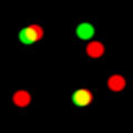
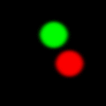
Red and green
Colocalization refers to different data analysis methods to characterize the degree of overlap between two channels in an image (conventionally called R and G channels, or red and green channels, independently of the WaveLength they have actually registered). A typical application in fluorescence microscopy is to study the presence of two labeled targets in the same region of a cell.
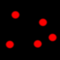
When viewed in an RGB representation, the overlap of red and green displays as yellow. Whenever you see yellow in the images below, you have colocalizing signals.
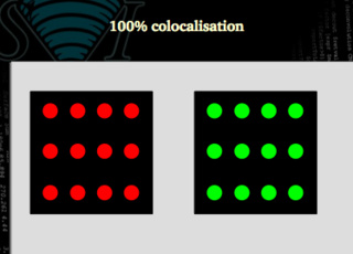
100% colocalization
We need to define some statistical figures that properly describe situations like these. Our coefficients must say that a situation like the following one is 100% colocalization:
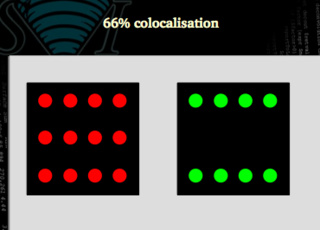
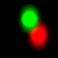
66 % colocalization
In this case, only 66% of the signal is colocalized.
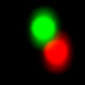
Is this case the same 66% as this other one?
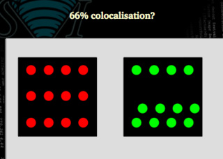
Clearly not. We may need to use figures that are able to distinguish between both situations. In the first case all the green signal is colocalized with the red one, but only 66 % of the red matches the green. In the second case, both signals are 66% colocalized.
We need coefficients that...
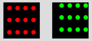
...are sensitive to the addition of extra non-colocalized signal:

...are insensitive to relative variations of intensities (for example if the power of one of the lasers is less than the other's):

...are insensitive to the presence of a Background (due to an acquisition offset or non specific staining, for example):
Coefficients and maps
The colocalization coefficients are figures that parametrize the degree of colocalization of the full two-channel image. On the other hand, maps parametrize the level of colocalization locally. In a map, a single colocalization value is calculated per VoXel creating a 3D distribution that can be represented in a 3D image.
See Colocalization Map.
Most common coefficients
The Pearson coefficient provides a measure of how well two signals are related by a linear equation, independently of what is the actual relationship. See Pearsons Interpretation.
On the other hand, the Manders coefficients provide information on how one particular channel matches the other one, separating the information. See Colocalization Theory.
Effects of imaging conditions
During image acquisition in a Fluorescence Microscope many things can go wrong, but even in the best experimental conditions there are two sources of degradation that are physically unavoidable:
- Photon Noise, due to the intrinsic nature of photons, and
- blur caused by diffraction.
Read Image Formation to see how diffraction, resolution and Numerical Aperture are related.
Let us take a closer look at two nearby signals. In the following examples a red and a green feature are not overlaping, but colocalization is very much affected by...
Blur
The blur around the features provides fake colocalizing signal.

Noise
Apart from this blur, the Photon Noise will cause signal fluctuations that will affect the analysis.
Background
On top of that, Backgrounds in the two channels will increase the colocalization levels dramatically.
Color shift
Misalignment of the detectors (Color Shift) will spoil colocalization, or even introduce fake one.
Cross-talk
If some signal is detected with the wrong detector (Cross Talk) fake colocalization will happen.
Example
Images below show improved separation of the red and green channel by deconvolution, which prevents false colocalization analysis from being included in the quantification.
Read more in Colocalization Theory.