
REDIRECT plugin: redirect loop detected!
Point spread function: theoretical vs. experimental
Benefits of using an experimental PSF
A theoretically calculated Point Spread Function (PSF) is a very good model of the imaging process in your microscope whenever this is ideally aligned and configured. Any deviation from the ideal conditions can have severe consequences on the quality of your image. Still, if you manage to measure the real PSF of your microscope, your image can be very well restored by Doing Deconvolution.
The best PSF is therefore the one you measure experimentally, in a sort of calibration of your microscope. It will include all the physical deviations from the ideal model, and your Image Restorations would be much better. See Experimental Psf.
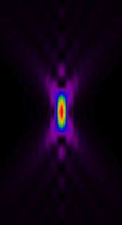
The following images show the theoretical and the experimental PSFs of a specific LSM 510 Confocal Microscope setup, using a 1.4 Numerical Aperture plan apo objective with oil as Lens Immersion Medium. The images are XY, XZ and YZ slices across the center of the images, in false color mode. The inset reference scale is 500 nm in length.
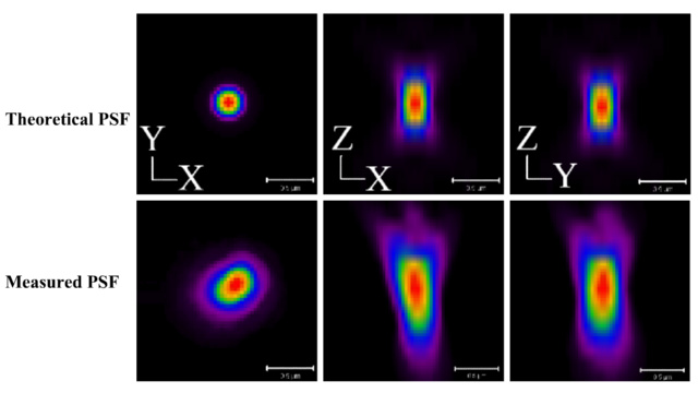
Images courtesy of Louis Villeneuve, Institut de Cardiologie de Montreal.
The experimental PSF shows noticeable differences when compared with the ideal one, namely a larger size and a loss of symmetry. Any image acquired with this setup will suffer from extra distortions that the ideal PSF can not account for.
The following images show the raw and deconvolved images of a fluorescent latex bead of 170 nm in diameter. Acquisition was made using the same LSM 510 microscope. VoXel size was about 40 x 40 x 160 nm (XYZ), averaging two times. (Excitation Wavelength: 540 nm, Emission Wavelength: 560 nm).
Row A shows the raw dataset, row B shows the deconvolution result using a theoretical PSF, while row C is the result with an experimental PSF.
The first three columns are XY, XZ and YZ slices across the center of the images, in false color mode. The inset reference scale is 500 nm in length.
The last column shows 3D visualizations of the datasets using the Huygens' Sfp Renderer.
The quality of the restoration in the latter case is noticeable.
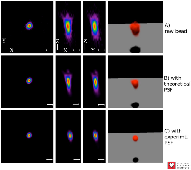
Images courtesy of Louis Villeneuve, Institut de Cardiologie de Montreal.
You can find out how the theoretical PSF of your particular setup looks like by using the online Nyquist Calculator.
Difficulties in practice
One user sent the following email:
We have been testing Huygens Professional with our data, using both the theoretical -on the fly- method as well as a measured PSF from 200 nm beads. I found that our data for some inexplicable reason gets smoothed too much using the measured PSF. Small structures such as dendritic spines (receiving ends of the dendrites of neurons) disappear using the average bead PSF. ...
Measuring the PSF
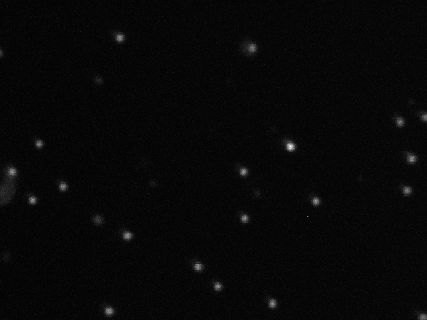
They have sent a Well Sampled, non clipped image of some beads to construct an Experimental Psf.
This is the MIP of the bead image, it looks pretty nice:
This is the final obtained Experimental Psf:
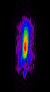
Full-width at half-maximum (FWHM), or Half Intensity Width (HIW): along Z axis: ~ 3200 nm, along the X axis: ~ 500 nm.
You can compare it with the Theoretical Psf for these conditions:
FWHM (HIW): ~ 1200 nm along Z, ~ 275 nm along X.
The theoretical one is almost one third in size!!! In our experience microscope are rarely as bad as that... Maybe there is an error in the beads sampling data, or the beads are larger than reported? If indeed the size of the PSF was overestimated, that would explain the reported vanishing details.
The image of the beads probably does not correspond to the conditions of the image of interest. We suspect it may be related with the sampling rate parameters, that may be wrong, so we obtain a reconstructed PSF much larger than expected.
To make a perfect DeConvolution, the following points must be taken into account:
- Recording Beads to obtain an experimental PSF should be done under exactly the same conditions as with the image of interest to be restored. The PSF is like the calibration of the optical system. In this case, we have a small WaveLength mismatch and, more important, a high Sampling Distances mismatch between the beads and the object of interest. (See also Parameter Variation).
- Clipped Images must be avoided, at least in the regions of interest. Otherwise deconvolution is useless, because clipping implies information loss.
- To capture all the image details, sampling rate must not be in any case above the Nyquist Rate.
- Much careful must be put in correctly recording all the image Microscopic Parameters, to avoid confusions.